Datei:Speed of sound in water.svg

Größe der PNG-Vorschau dieser SVG-Datei: 720 × 540 Pixel. Weitere Auflösungen: 320 × 240 Pixel | 640 × 480 Pixel | 1.024 × 768 Pixel | 1.280 × 960 Pixel | 2.560 × 1.920 Pixel.
Originaldatei (SVG-Datei, Basisgröße: 720 × 540 Pixel, Dateigröße: 36 KB)
Beschreibung
| Beschreibung |
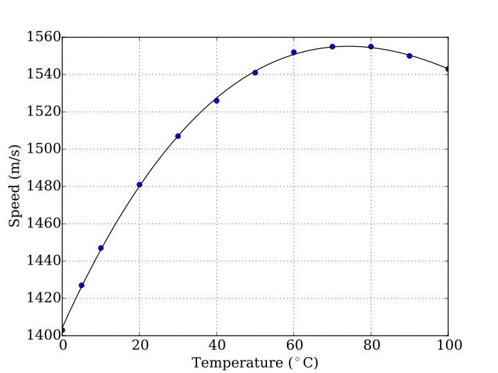
English: Graph of the speed of sound in water vs temperature. Tabulated values (circle markers) from "The Engineering Toolbox" [1].
Smooth continuous line is a 3rd degree polynomial fit (see below) calculated on the tabulated data, accurate within 0.1%.
Español: Gráfico de la rapidez del sonido en el agua versus temperatura. Los datos tabulados (círculos) se obtuvieron de "The Egineering Toolbox" [2].
La línea continua es un ajuste polinomial de orden 3 (ver abajo) calculado a partir de los datos tabulados, la precisión es del 0.1%.
C(T) = a0 + a1T + a2T2 + a3T3 (m/s) """
Plot of the speed of sound versus temperature in water
The data is obtained from "The Engineering Toolbox" [1]_
References
----------
.. [1] The Engineering Toolbox. Water - Speed of Sound.
Accesed: April 27, 2015.
http://www.engineeringtoolbox.com/sound-speed-water-d_598.html
"""
import numpy as np
import matplotlib.pyplot as plt
from matplotlib import rcParams
rcParams['font.family'] = 'serif'
rcParams['font.size'] = 16
data = np.array([
[ 0., 1403.],
[ 5., 1427.],
[ 10., 1447.],
[ 20., 1481.],
[ 30., 1507.],
[ 40., 1526.],
[ 50., 1541.],
[ 60., 1552.],
[ 70., 1555.],
[ 80., 1555.],
[ 90., 1550.],
[ 100., 1543.]])
temp = data[:, 0]
vel = data[:, 1]
a3, a2, a1, a0 = np.polyfit(temp, vel, 3)
temp_fit = np.linspace(0,100)
vel_fit = a0 + a1*temp_fit + a2*temp_fit**2 + a3*temp_fit**3
plt.plot(temp, vel, 'o')
plt.plot(temp_fit, vel_fit, 'k')
plt.grid(True)
plt.xlabel(r"Temperature ($^\circ$C)")
plt.ylabel(r"Speed (m/s)")
plt.savefig("Speed_of_sound_in_water.svg")
|
| Datum | |
| Quelle | Eigenes Werk |
| Urheber | K. Krallis, SV1XV |
Lizenz
Diese Datei ist unter der Creative-Commons-Lizenz „Namensnennung 1.0 generisch“ (US-amerikanisch) lizenziert.
- Dieses Werk darf von dir
- verbreitet werden – vervielfältigt, verbreitet und öffentlich zugänglich gemacht werden
- neu zusammengestellt werden – abgewandelt und bearbeitet werden
- Zu den folgenden Bedingungen:
- Namensnennung – Du musst angemessene Urheber- und Rechteangaben machen, einen Link zur Lizenz beifügen und angeben, ob Änderungen vorgenommen wurden. Diese Angaben dürfen in jeder angemessenen Art und Weise gemacht werden, allerdings nicht so, dass der Eindruck entsteht, der Lizenzgeber unterstütze gerade dich oder deine Nutzung besonders.
Dateiversionen
Klicke auf einen Zeitpunkt, um diese Version zu laden.
| Version vom | Vorschaubild | Maße | Benutzer | Kommentar | |
|---|---|---|---|---|---|
| aktuell | 23:16, 27. Apr. 2015 | | 720 × 540 (36 KB) | wikimediacommons>Nicoguaro | Similar formatting to other plots in the article. Added Python code (and data) for the automatic generation of the file. |
Dateiverwendung
Die folgende Seite verwendet diese Datei: